BeerKan experiment and the BEST algorithm

library(tidysoilinfiltration)
library(dplyr)
library(tibble)
library(ggplot2)

Overview

The BeerKan (Beerkan Estimation of Soil Transfer parameters) protocol is a low-cost field method: a fixed volume of water is poured repeatedly inside a ring, and the time for each pour to completely infiltrate is recorded. Unlike standard ring or Minidisk methods, measurement proceeds at zero pressure head (ponded).

The BEST algorithm (Lassabatère et al., 2006) fits the Haverkamp et al. (1994) quasi-exact implicit infiltration model to the resulting I(t) series, recovering both the saturated hydraulic conductivity Ks and the sorptivity S. The Van Genuchten scale parameter α is then recovered analytically.

Step	Function
Pour events → cumulative I(t)	beerkan_cumulative()
VG shape params (n, α)	infiltration_vg_params(..., suction = 0)
Philip quick estimate	fit_infiltration()
BEST: Ks, S, α	fit_best()

---

1. Field data

A BeerKan run pours a fixed 100 mL of water 10 times into a ring (radius 5 cm), recording how long each pour takes to disappear.

run <- tibble(
  pour   = 1:10,
  volume = 100,                                     # mL per pour
  time   = c(12, 18, 25, 30, 33, 34, 35, 35, 36, 35)  # s to infiltrate
)
run
#> # A tibble: 10 × 3
#>     pour volume  time
#>    <int>  <dbl> <dbl>
#>  1     1    100    12
#>  2     2    100    18
#>  3     3    100    25
#>  4     4    100    30
#>  5     5    100    33
#>  6     6    100    34
#>  7     7    100    35
#>  8     8    100    35
#>  9     9    100    36
#> 10    10    100    35

The infiltration time increases early on (soil is initially dry) then stabilises near 35 s as the soil approaches steady state.

---

2. Cumulative infiltration

beerkan_cumulative() accumulates both time and volume, then converts to depth using the ring area.

cum <- beerkan_cumulative(run, volume_col = volume, time_col = time, radius = 5)
cum |> select(pour, volume, time, .cumulative_time, .infiltration)
#> # A tibble: 10 × 5
#>     pour volume  time .cumulative_time .infiltration
#>    <int>  <dbl> <dbl>            <dbl>         <dbl>
#>  1     1    100    12               12          1.27
#>  2     2    100    18               30          2.55
#>  3     3    100    25               55          3.82
#>  4     4    100    30               85          5.09
#>  5     5    100    33              118          6.37
#>  6     6    100    34              152          7.64
#>  7     7    100    35              187          8.91
#>  8     8    100    35              222         10.2 
#>  9     9    100    36              258         11.5 
#> 10    10    100    35              293         12.7

ggplot(cum, aes(x = .cumulative_time, y = .infiltration)) +
  geom_point() +
  geom_line() +
  labs(title = "Cumulative BeerKan infiltration",
       x = "Cumulative time (s)", y = "Infiltration depth (cm)")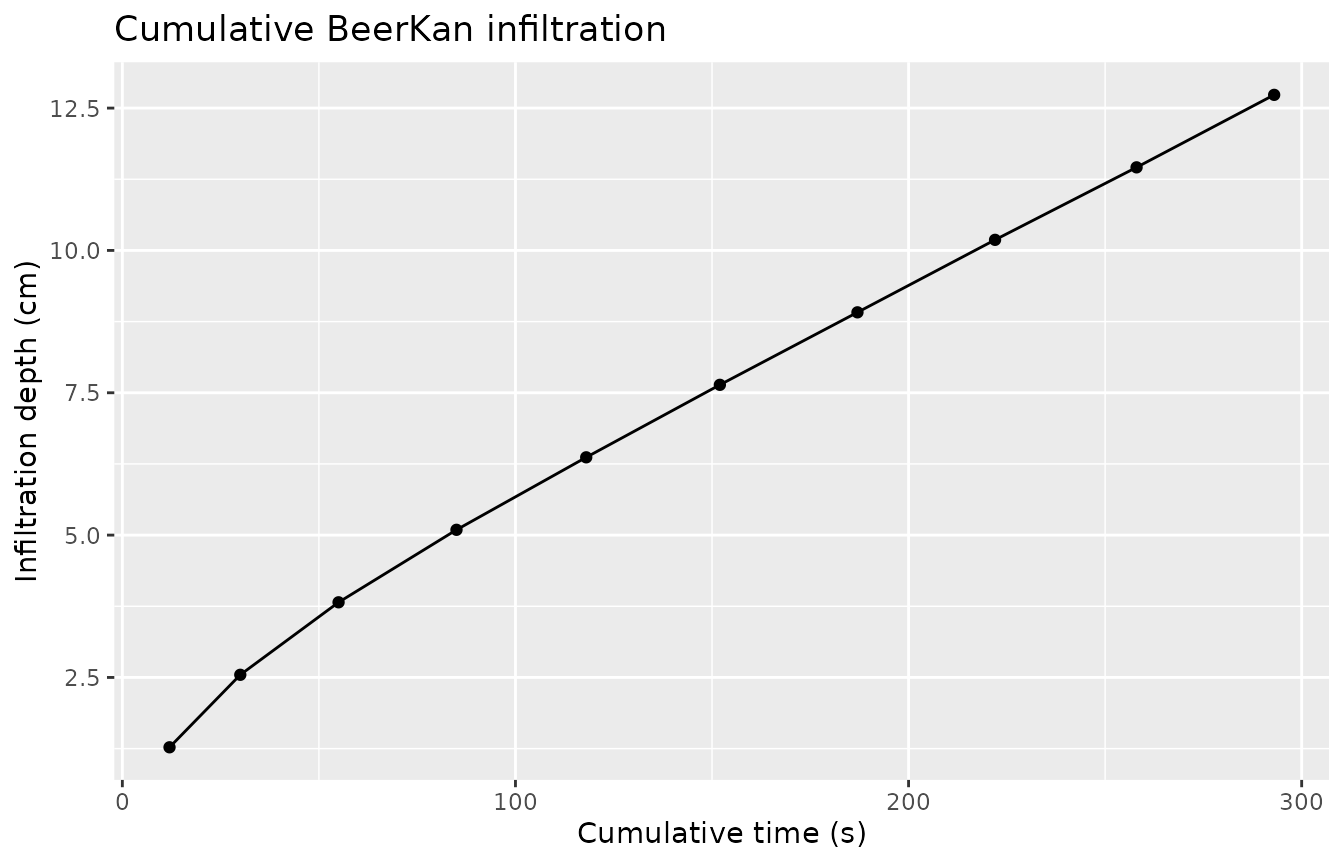

The curve transitions from a rapid early phase to a linear steady-state, consistent with the Haverkamp model.

---

3. VG shape parameters from texture

For BEST we need the Van Genuchten shape parameter n. Since the experiment runs at zero pressure head, use suction = 0 to retrieve only the shape parameters (.A will be NA, which is expected):

soil_meta <- tibble(texture = "loam", theta_s = 0.43, theta_i = 0.12) |>
  infiltration_vg_params(texture = texture, suction = 0)

soil_meta |> select(texture, theta_s, theta_i, .n, .alpha, .A)
#> # A tibble: 1 × 6
#>   texture theta_s theta_i    .n .alpha    .A
#>   <chr>     <dbl>   <dbl> <dbl>  <dbl> <dbl>
#> 1 loam       0.43    0.12  1.56  0.036    NA

---

4. Philip quick estimate

Before running BEST, a quick Philip two-term fit gives a preliminary sorptivity and conductivity proxy.

philip <- fit_infiltration(cum,
                           infiltration_col = .infiltration,
                           sqrt_time_col    = .sqrt_time)
philip
#> # A tibble: 1 × 5
#>     .C2    .C1 .C2_std_error .C1_std_error .convergence
#>   <dbl>  <dbl>         <dbl>         <dbl> <lgl>       
#> 1 0.343 0.0235        0.0298       0.00141 TRUE

C₁ (0.0235 cm/s) is a rough Ks proxy; BEST will refine this using the full Haverkamp model.

---

5. BEST algorithm

fit_best() accepts the cumulative I(t) data together with the soil moisture parameters (theta_s, theta_i) and the VG shape exponent n.

best <- fit_best(
  cum,
  infiltration_col = .infiltration,
  time_col         = .cumulative_time,
  theta_s          = 0.43,
  theta_i          = 0.12,
  n                = soil_meta$.n
)
best
#> # A tibble: 1 × 7
#>      .Ks    .S .alpha .Ks_std_error .S_std_error .steady_n .convergence
#>    <dbl> <dbl>  <dbl>         <dbl>        <dbl>     <int> <lgl>       
#> 1 0.0360 0.261   1.24      0.000144      0.00215         4 TRUE

The key outputs:

Parameter	Symbol	Value	Units
Saturated hydraulic conductivity	Ks	0.036	cm/s
Sorptivity	S	0.261	cm/s^0.5
VG scale parameter	α	1.24	1/cm

---

6. Comparing BEST methods

Three fitting strategies are available. "steady" (default) uses the last steady_n = 4 points to define the steady-state window; "slope" uses the early-time transient to estimate S independently.

methods <- c("steady", "slope", "intercept")

results <- lapply(methods, function(m) {
  fit_best(
    cum,
    infiltration_col = .infiltration,
    time_col         = .cumulative_time,
    theta_s = 0.43, theta_i = 0.12,
    n       = soil_meta$.n,
    method  = m
  ) |>
    mutate(method = m)
}) |>
  bind_rows()

results |> select(method, .Ks, .S, .alpha, .convergence)
#> # A tibble: 3 × 5
#>   method       .Ks    .S .alpha .convergence
#>   <chr>      <dbl> <dbl>  <dbl> <lgl>       
#> 1 steady    0.0360 0.261  1.24  TRUE        
#> 2 slope     0.0360 0.569  0.261 TRUE        
#> 3 intercept 0.0360 0.261  1.24  TRUE

---

7. Multi-site workflow

For field campaigns, group by site and process all runs together.

# Per-site soil parameters are embedded as columns so fit_best() can resolve
# them via tidy evaluation within each group.
field_runs <- tibble(
  site    = rep(c("S1", "S2"), each = 10),
  pour    = rep(1:10, 2),
  volume  = 100,
  time    = c(
    12, 18, 25, 30, 33, 34, 35, 35, 36, 35,   # S1 — loam
     8, 11, 14, 17, 19, 20, 20, 21, 20, 21    # S2 — sandy loam (faster)
  ),
  theta_s = rep(c(0.43, 0.40), each = 10),
  theta_i = rep(c(0.12, 0.08), each = 10),
  n       = rep(c(1.56, 1.89), each = 10)
)

multi_cum <- field_runs |>
  group_by(site) |>
  beerkan_cumulative(volume_col = volume, time_col = time, radius = 5)

multi_best <- multi_cum |>
  group_by(site) |>
  fit_best(
    infiltration_col = .infiltration,
    time_col         = .cumulative_time,
    theta_s          = theta_s,
    theta_i          = theta_i,
    n                = n
  )

multi_best |> select(site, .Ks, .S, .alpha, .convergence)
#> # A tibble: 2 × 5
#>   site     .Ks    .S .alpha .convergence
#>   <chr>  <dbl> <dbl>  <dbl> <lgl>       
#> 1 S1    0.0360 0.261   1.24 TRUE        
#> 2 S2    0.0618 0.359   1.21 TRUE

Site S2 (sandy loam) shows higher Ks, consistent with its coarser texture and faster infiltration times.

---

References

Haverkamp, R., Ross, P. J., Smettem, K. R. J., & Parlange, J.-Y. (1994). Three-dimensional analysis of infiltration from the disc infiltrometer: 2. Physically based infiltration equation. Water Resources Research, 30(11), 2931–2935.

Lassabatère, L., Angulo-Jaramillo, R., Soria Ugalde, J. M., Cuenca, R., Braud, I., & Haverkamp, R. (2006). Beerkan estimation of soil transfer parameters through infiltration experiments—BEST. Soil Science Society of America Journal, 70(2), 521–532. https://doi.org/10.2136/sssaj2005.0026