Minidisk tension-disc infiltrometer workflow

library(tidysoilinfiltration)
library(dplyr)
library(tibble)
library(ggplot2)

Overview

The Minidisk Infiltrometer (Decagon Devices) delivers water at a controlled tension (suction) below saturation. The Zhang (1997) method extracts the unsaturated hydraulic conductivity K(h) from a two-step analysis:

Fit the Philip (1957) two-term polynomial to cumulative infiltration to recover the conductivity proxy C₁.
Divide C₁ by the soil-specific shape parameter A (derived from Van Genuchten parameters and the applied tension) to get K(h).

minidisk_conductivity() wraps steps 2 in a single call, giving a four-step pipeline from raw field readings to K(h):

Step	Function
Raw readings → I(t)	`infiltration_cumulative()`
Philip two-term fit → C₁	`fit_infiltration()`
VG lookup + K(h) = C₁ / A	`minidisk_conductivity()`

The underlying functions infiltration_vg_params(), parameter_A_zhang(), and hydraulic_conductivity_minidisk() remain exported for cases that need more control.

1. Single-site example

A typical Minidisk run records the reservoir volume (mL) at fixed time intervals. The disc radius is 2.25 cm (the standard instrument).

raw <- tibble(
  time   = seq(0, 300, 30),   # seconds
  volume = c(95, 89, 86, 83, 80, 77, 74, 73, 71, 69, 67)  # mL
)

The full pipeline from raw readings to K(h):

result <- raw |>
  infiltration_cumulative(time = time, volume = volume) |>
  fit_infiltration(.infiltration, .sqrt_time) |>
  minidisk_conductivity(texture = "sandy loam", suction = 2)

result |> select(.C1, .n, .alpha, .A, .K_h)
#> # A tibble: 1 × 5
#>       .C1    .n .alpha    .A     .K_h
#>     <dbl> <dbl>  <dbl> <dbl>    <dbl>
#> 1 0.00252  1.89  0.075  3.91 0.000645

K(h) ≈ 6.45^{-4} cm/s at 2 cm tension for this sandy loam sample.

2. Multi-site workflow

For field campaigns with multiple samples, group by site before infiltration_cumulative(). Because grouping is now preserved through cumulative calculations, only one group_by() is needed for the whole pipeline.

multi <- tibble(
  site   = rep(c("A", "B"), each = 11),
  time   = rep(seq(0, 300, 30), 2),
  volume = c(
    95, 89, 86, 83, 80, 77, 74, 73, 71, 69, 67,   # site A — sandy loam
    95, 87, 81, 76, 72, 68, 65, 63, 61, 59, 58    # site B — loamy sand
  )
)

# Per-site metadata (texture, suction)
meta <- tibble(
  site    = c("A", "B"),
  texture = c("sandy loam", "loamy sand"),
  suction = c(2, 2)
)

multi_result <- multi |>
  group_by(site) |>
  infiltration_cumulative(time = time, volume = volume) |>
  fit_infiltration(.infiltration, .sqrt_time) |>
  left_join(meta, by = "site") |>
  minidisk_conductivity(texture = texture, suction = suction)

multi_result |> select(site, texture, .C1, .A, .K_h)
#> # A tibble: 2 × 5
#>   site  texture        .C1    .A     .K_h
#>   <chr> <chr>        <dbl> <dbl>    <dbl>
#> 1 A     sandy loam 0.00252  3.91 0.000645
#> 2 B     loamy sand 0.00137  2.43 0.000565

3. Analytical A with `method = "zhang"`

For non-standard disc radii or suction levels outside the Decagon table, pass method = "zhang" to compute A analytically from Zhang (1997) rather than looking it up. The radius argument is only used in this mode.

multi |>
  group_by(site) |>
  infiltration_cumulative(time = time, volume = volume) |>
  fit_infiltration(.infiltration, .sqrt_time) |>
  left_join(meta, by = "site") |>
  minidisk_conductivity(texture = texture, suction = suction,
                        method = "zhang", radius = 2.25) |>
  select(site, texture, .A, .K_h)
#> # A tibble: 2 × 4
#>   site  texture       .A     .K_h
#>   <chr> <chr>      <dbl>    <dbl>
#> 1 A     sandy loam  3.82 0.000660
#> 2 B     loamy sand  4.21 0.000326

The analytical A values will differ slightly from the tabulated ones — both approaches are valid; the choice depends on whether your suction and radius match the Decagon reference conditions.

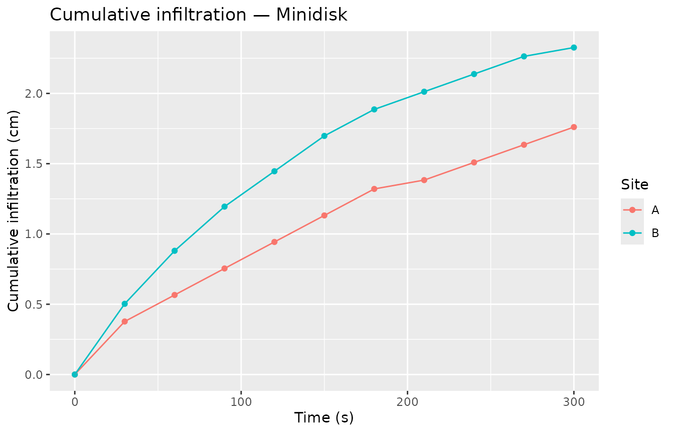
4. Visualisation

multi |>
  group_by(site) |>
  infiltration_cumulative(time = time, volume = volume) |>
  ggplot(aes(x = time, y = .infiltration, colour = site)) +
  geom_point() +
  geom_line() +
  labs(
    title  = "Cumulative infiltration — Minidisk",
    x      = "Time (s)",
    y      = "Cumulative infiltration (cm)",
    colour = "Site"
  )

References

Decagon Devices, Inc. (2005). Mini Disk Infiltrometer User’s Manual.

Philip, J. R. (1957). The theory of infiltration: 4. Sorptivity and algebraic infiltration equations. Soil Science, 84(3), 257–264.