Fitting diagnostics: convergence, residuals, and uncertainty

library(tidysoilwater)
library(dplyr)
library(tibble)
library(ggplot2)

Overview

fit_swrc() returns a convergence flag and standard errors alongside the fitted parameters. This vignette shows how to:

1. Check and handle non-converged fits
2. Plot residuals to detect systematic model misfit
3. Interpret parameter standard errors and compute confidence intervals
4. Understand starting-value sensitivity, particularly for clay soils

---

1. Detecting non-converged fits

The convergence column is TRUE when nls() converged and FALSE (with NA parameters) when it did not.

set.seed(2947)

# Reference parameters for three soil types
soils <- tribble(
  ~soil,          ~theta_r, ~theta_s, ~alpha,   ~n,
  "sandy loam",      0.047,    0.430,  0.145, 2.68,
  "loam",            0.078,    0.430,  0.036, 1.56,
  "silty clay loam", 0.089,    0.430,  0.010, 1.23   # difficult for NLS
)

heads   <- c(0, 10, 33, 100, 330, 1000, 3300, 5000, 15000)
sigma   <- 0.005

# Generate synthetic observations
obs <- soils |>
  tidyr::crossing(h = heads) |>
  mutate(
    m     = 1 - 1 / n,
    theta_true = theta_r + (theta_s - theta_r) /
                   (1 + (alpha * h)^n)^m,
    theta = pmax(0.01, theta_true + rnorm(n(), 0, sigma))
  ) |>
  select(soil, h, theta)

fits <- obs |>
  group_by(soil) |>
  fit_swrc(theta_col = theta, h_col = h)

fits |>
  select(soil, theta_r, theta_s, alpha, n, convergence)
#> # A tibble: 3 × 6
#>   soil            theta_r theta_s   alpha     n convergence
#>   <chr>             <dbl>   <dbl>   <dbl> <dbl> <lgl>      
#> 1 loam             0.0731   0.429 0.0349   1.54 TRUE       
#> 2 sandy loam       0.0469   0.431 0.141    2.71 TRUE       
#> 3 silty clay loam  0.0298   0.427 0.00854  1.19 TRUE

n_failed <- sum(!fits$convergence)
cat(sprintf("%d / %d fits converged.\n", sum(fits$convergence), nrow(fits)))
#> 3 / 3 fits converged.

if (n_failed > 0) {
  cat("\nNon-converged soils:\n")
  fits |>
    filter(!convergence) |>
    pull(soil) |>
    cat(sep = "\n")
}

What to do when a fit fails:

• Try different starting values (see Section 4)
• Add more observations near the dry end (high |h|) where the curve flattens
• For very fine-textured soils (n < 1.2), consider fixing θ_s from bulk density measurements and fitting only θ_r, α, n

---

2. Residual analysis

A good fit should show residuals scattered randomly around zero. Systematic patterns suggest model misfit or bad observations.

# Reconstruct fitted curves and compute residuals
predicted <- fits |>
  select(soil, theta_r, theta_s, alpha, n) |>
  filter(!is.na(theta_r)) |>
  tidyr::crossing(h = heads) |>
  mutate(m = 1 - 1 / n) |>
  swrc_van_genuchten(theta_r = theta_r, theta_s = theta_s,
                     alpha = alpha, n = n, h = h) |>
  rename(theta_fitted = .theta)

resid_df <- obs |>
  left_join(predicted |> select(soil, h, theta_fitted),
            by = c("soil", "h")) |>
  filter(!is.na(theta_fitted)) |>
  mutate(residual = theta - theta_fitted)

ggplot(resid_df, aes(x = h, y = residual, colour = soil)) +
  geom_hline(yintercept = 0, linetype = "dashed", colour = "grey60") +
  geom_point(size = 2) +
  scale_x_log10(labels = scales::label_comma()) +
  facet_wrap(~soil) +
  labs(
    x     = "Matric potential |h| (cm)",
    y     = expression(theta[obs] - theta[fit]),
    title = "Residuals by soil type"
  ) +
  theme(legend.position = "none")
#> Warning in scale_x_log10(labels = scales::label_comma()): log-10
#> transformation introduced infinite values.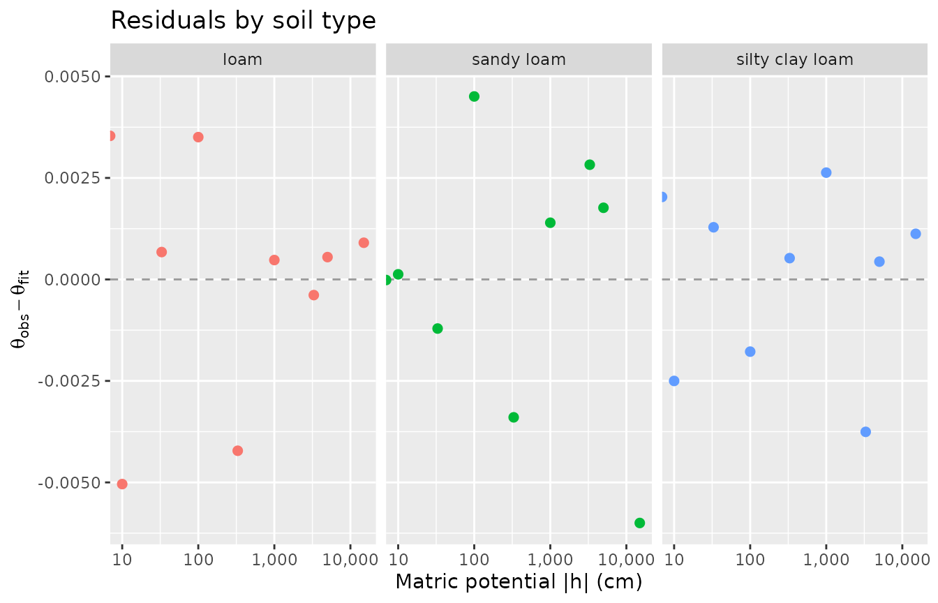

resid_df |>
  group_by(soil) |>
  summarise(
    RMSE  = sqrt(mean(residual^2)),
    MAE   = mean(abs(residual)),
    max_e = max(abs(residual))
  )
#> # A tibble: 3 × 4
#>   soil               RMSE     MAE   max_e
#>   <chr>             <dbl>   <dbl>   <dbl>
#> 1 loam            0.00279 0.00214 0.00504
#> 2 sandy loam      0.00303 0.00236 0.00600
#> 3 silty clay loam 0.00205 0.00179 0.00375

---

3. Parameter standard errors and confidence intervals

fit_swrc() returns standard errors for all four parameters. For approximate 95% CIs use ± 2 SE; for exact intervals use confint() on the nls object directly (see note below).

fits |>
  filter(convergence) |>
  select(soil, theta_r, std_error_theta_r, alpha, std_error_alpha, n, std_error_n)
#> # A tibble: 3 × 7
#>   soil       theta_r std_error_theta_r   alpha std_error_alpha     n std_error_n
#>   <chr>        <dbl>             <dbl>   <dbl>           <dbl> <dbl>       <dbl>
#> 1 loam        0.0731           0.00450 0.0349          0.00264  1.54      0.0332
#> 2 sandy loam  0.0469           0.00176 0.141           0.00662  2.71      0.148 
#> 3 silty cla…  0.0298           0.0464  0.00854         0.00118  1.19      0.0372

# 95 % CI: estimate ± 1.96 × SE
fits |>
  filter(convergence) |>
  mutate(
    n_lo = n - 1.96 * std_error_n,
    n_hi = n + 1.96 * std_error_n
  ) |>
  select(soil, n, n_lo, n_hi, std_error_n)
#> # A tibble: 3 × 5
#>   soil                n  n_lo  n_hi std_error_n
#>   <chr>           <dbl> <dbl> <dbl>       <dbl>
#> 1 loam             1.54  1.48  1.61      0.0332
#> 2 sandy loam       2.71  2.41  3.00      0.148 
#> 3 silty clay loam  1.19  1.11  1.26      0.0372

Interpretation:

• Narrow SE relative to estimate → parameter is well-constrained by the data
• SE larger than ~25% of estimate → consider adding observations at extremes of the retention curve (very wet or very dry)
• The n parameter typically has the smallest relative SE when the data span a wide pressure range (several log-cycles)

---

4. Starting value sensitivity

Default starting values (θ_r = 0.9 × min(θ), θ_s = 1.05 × max(θ), α = 0.1, n = 2.0) work well for most mineral soils with n ≥ 1.4. Clay soils (n ≈ 1.1–1.3) can require tighter, soil-specific starts.

# Difficult clay loam: n ≈ 1.23
clay_obs <- obs |> filter(soil == "silty clay loam")

# Strategy: grid search over (alpha, n) starting points
start_grid <- expand.grid(
  alpha_start = c(0.005, 0.01, 0.02, 0.05),
  n_start     = c(1.1, 1.3, 1.5, 2.0)
)

fit_with_start <- function(a0, n0, obs_df) {
  theta_vec <- obs_df$theta
  h_vec     <- abs(obs_df$h)

  tryCatch({
    fit <- nls(
      theta ~ theta_r + (theta_s - theta_r) /
                (1 + (alpha * h_vec)^n)^(1 - 1/n),
      data  = list(theta = theta_vec, h_vec = h_vec),
      start = list(theta_r = min(theta_vec) * 0.9,
                   theta_s = max(theta_vec) * 1.05,
                   alpha   = a0,
                   n       = n0),
      control = nls.control(maxiter = 200)
    )
    broom::tidy(fit) |>
      tidyr::pivot_wider(names_from = term, values_from = estimate) |>
      mutate(alpha_start = a0, n_start = n0, converged = TRUE)
  },
  error = function(e)
    tibble(alpha_start = a0, n_start = n0, converged = FALSE)
  )
}

start_results <- purrr::map2_dfr(
  start_grid$alpha_start,
  start_grid$n_start,
  fit_with_start,
  obs_df = clay_obs
)

start_results |>
  select(alpha_start, n_start, converged, alpha, n) |>
  arrange(desc(converged), n_start)
#> # A tibble: 52 × 5
#>    alpha_start n_start converged    alpha     n
#>          <dbl>   <dbl> <lgl>        <dbl> <dbl>
#>  1       0.005     1.1 TRUE      NA       NA   
#>  2       0.005     1.1 TRUE      NA       NA   
#>  3       0.005     1.1 TRUE       0.00854 NA   
#>  4       0.005     1.1 TRUE      NA        1.19
#>  5       0.01      1.1 TRUE      NA       NA   
#>  6       0.01      1.1 TRUE      NA       NA   
#>  7       0.01      1.1 TRUE       0.00854 NA   
#>  8       0.01      1.1 TRUE      NA        1.19
#>  9       0.005     1.3 TRUE      NA       NA   
#> 10       0.005     1.3 TRUE      NA       NA   
#> # ℹ 42 more rows

Key recommendations for clay soils

1. α starting point: use 0.005–0.02 (reflecting fine-textured pores)
2. n starting point: stay in the expected range 1.1–1.3 rather than defaulting to 2.0
3. Data requirements: at minimum 8–10 observations spanning pF 0–4.2; include at least two points between pF 2–3 where clay SWRCs bend
4. Fixed parameters: if K_sat is measured, pass it as θ_s constraint; reduces the fitting problem to three parameters

---

5. Visualising fitted curves alongside observations

# Only converged soils
fit_curves <- fits |>
  filter(convergence) |>
  select(soil, theta_r, theta_s, alpha, n) |>
  tidyr::crossing(h = 10^seq(0, 5, by = 0.1)) |>
  mutate(m = 1 - 1 / n) |>
  swrc_van_genuchten(theta_r = theta_r, theta_s = theta_s,
                     alpha = alpha, n = n, h = h)

ggplot() +
  geom_line(data  = fit_curves,
            aes(x = h, y = .theta, colour = soil),
            linewidth = 0.9) +
  geom_point(data = obs |> filter(soil != "silty clay loam"),
             aes(x = h, y = theta, colour = soil),
             size = 2.5) +
  scale_x_log10(labels = scales::label_comma()) +
  labs(
    x      = "Matric potential |h| (cm)",
    y      = expression(theta~(m^3/m^3)),
    colour = "Soil",
    title  = "Observed (points) vs fitted VG curves"
  )
#> Warning in scale_x_log10(labels = scales::label_comma()): log-10
#> transformation introduced infinite values.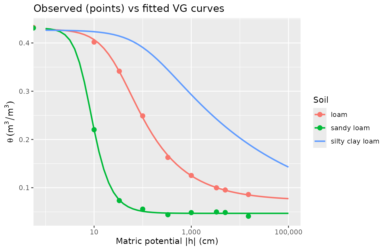

---

Summary

Diagnostic	What to check
convergence column	FALSE → adjust starting values or data range
Residual plot	Systematic patterns → model misfit; outliers → bad observations
std_error_* columns	SE / estimate > 0.25 → more data needed
Starting value grid	Clay soils: try α ∈ [0.005, 0.02], n ∈ [1.1, 1.3]