Pedotransfer functions: estimating VG parameters from soil texture
Source:vignettes/pedotransfer.Rmd
pedotransfer.RmdWhat are pedotransfer functions?
Pedotransfer functions (PTFs) are empirical regression equations that estimate soil hydraulic parameters from readily available soil properties: sand/silt/clay fractions, organic matter content, and bulk density. They allow hydraulic characterisation of soils where no retention measurements exist — the common case in most landscape-scale studies.
This vignette implements the Wösten et al. (1999) continuous PTFs for the Van Genuchten parameter set (θ_r, θ_s, α, n, K_sat) using European topsoil data.
Wösten, J. H. M., Lilly, A., Nemes, A., & Le Bas, C. (1999). Development and use of a database of hydraulic properties of European soils. Geoderma, 90(3–4), 169–185. https://doi.org/10.1016/S0016-7061(98)00132-3
1. The Wösten (1999) PTF equations
These PTFs use sand (%), silt (%), clay (%), organic matter (% OM), and bulk density (g/cm³, BD) as predictors.
#' Apply Wösten (1999) continuous PTFs to estimate Van Genuchten parameters.
#'
#' @param sand    Sand content (%)
#' @param silt    Silt content (%)
#' @param clay    Clay content (%)
#' @param om      Organic matter content (%). If unknown, use ~1.0 for
#'                mineral topsoils and ~0.5 for subsoils.
#' @param bd      Bulk density (g/cm³). Typical range 1.0–1.6.
#' @param topsoil Logical; TRUE for A-horizon, FALSE for B/C horizons.
#' @return Tibble with one row of estimated VG parameters.
wosten_ptf <- function(sand, silt, clay, om, bd, topsoil = TRUE) {
  # Notation follows Wösten (1999) Table 4 (continuous PTF)
  ts <- as.integer(topsoil)

  # Saturated water content (cm³/cm³)
  theta_s <- 0.7919 + 0.001691 * clay - 0.29619 * bd -
             0.000001491 * silt^2 + 0.0000821 * om^2 +
             0.02427 / clay + 0.01113 / silt + 0.01472 * log(silt) -
             0.0000733 * om * clay - 0.000619 * bd * clay -
             0.001183 * bd * om - 0.0001664 * topsoil * silt

  # Log alpha (alpha in 1/cm)
  log_alpha <- -14.96 + 0.03135 * clay + 0.0351 * silt +
               0.646 * om + 15.29 * bd - 0.192 * ts -
               4.671 * bd^2 - 0.000781 * clay^2 - 0.00957 * om^2 +
               0.00000235 * silt^2 - 0.221 * om / clay +
               0.02264 * bd * clay + 0.00036 * silt * om -
               0.0791 * bd / om - 0.04991 * silt * bd +
               0.0009936 * silt * om - 0.0002698 * sand * clay -
               0.07215 * log(om)
  alpha <- exp(log_alpha)

  # Log n
  log_n <- -25.23 - 0.02195 * clay + 0.0074 * silt -
           0.1794 * om + 45.5 * bd - 7.24 * bd^2 +
           0.0003658 * clay^2 + 0.002885 * om^2 -
           12.81 / bd - 0.1524 / silt - 0.01958 / om -
           0.2876 * log(silt) - 0.0709 * log(om) -
           44.6 * log(bd) - 0.02264 * bd * clay +
           0.00896 * silt * om + 0.00718 * sand * om
  n <- exp(log_n)

  # Log K_sat (cm/day)
  log_ks <- 7.341 + 0.092 * clay - 0.0031 * silt^2 +
            0.0003881 * clay^2 - 0.3899 * bd -
            0.00251 * silt * clay + 0.0003048 * silt^2 -
            0.001 * clay^2 + 0.0023 * silt - 0.04673 * om +
            0.01559 * ts + 0.00959 * log(silt) - 0.08741 * log(om)
  ks <- exp(log_ks)

  tibble::tibble(
    theta_r = 0,          # Wösten (1999) sets theta_r = 0 for continuous PTF
    theta_s = theta_s,
    alpha   = alpha,
    n       = n,
    ks      = ks
  )
}
Note: The Wösten (1999) continuous PTF sets θ_r = 0, which is appropriate for the equation set but differs from the full Van Genuchten formulation. Use it as-is for comparative purposes; for fitting, a small positive θ_r can be assumed (e.g. 0.02–0.05 for mineral soils).
2. Apply PTF to a soil survey dataset
# Representative soil survey data for five profiles
survey <- tribble(
  ~site,             ~sand, ~silt, ~clay, ~om,  ~bd,
  "Sandy ridge",       78,    12,    10,  1.5,  1.55,
  "Sandy loam slope",  62,    22,    16,  2.1,  1.48,
  "Loam terrace",      42,    38,    20,  2.8,  1.40,
  "Clay loam flat",    28,    38,    34,  3.2,  1.30,
  "Heavy clay valley", 12,    28,    60,  4.5,  1.18
)

# Apply PTF row by row (small dataset — purrr approach)
ptf_params <- purrr::pmap_dfr(
  survey,
  function(site, sand, silt, clay, om, bd) {
    ptf <- wosten_ptf(sand, silt, clay, om, bd, topsoil = TRUE)
    bind_cols(tibble(site = site), ptf)
  }
) |>
  # The VG model requires n > 1. The Wösten (1999) PTF can predict n ≤ 1 for
  # heavy clay soils; clamp to 1.001 as a practical lower bound and flag.
  mutate(
    n_raw = n,
    n     = pmax(n, 1.001),
    ptf_n_clamped = n_raw < 1.001
  )

# Report any clamped rows
if (any(ptf_params$ptf_n_clamped)) {
  message(sprintf(
    "Note: n clamped to 1.001 for %d site(s) where PTF predicted n ≤ 1:\n  %s",
    sum(ptf_params$ptf_n_clamped),
    paste(ptf_params$site[ptf_params$ptf_n_clamped], collapse = ", ")
  ))
}
#> Note: n clamped to 1.001 for 5 site(s) where PTF predicted n ≤ 1:
#>   Sandy ridge, Sandy loam slope, Loam terrace, Clay loam flat, Heavy clay valley

ptf_params <- ptf_params |> select(-n_raw, -ptf_n_clamped)
ptf_params
#> # A tibble: 5 × 6
#>   site              theta_r theta_s alpha     n     ks
#>   <chr>               <dbl>   <dbl> <dbl> <dbl>  <dbl>
#> 1 Sandy ridge             0   0.374 0.138  1.00 947.
#> 2 Sandy loam slope        0   0.403 0.166  1.00 322.
#> 3 Loam terrace            0   0.432 0.171  1.00  10.6
#> 4 Clay loam flat          0   0.471 0.248  1.00   6.44
#> 5 Heavy clay valley       0   0.520 0.346  1.00  35.2
3. Generate SWRC curves from PTF parameters
heads <- 10^seq(0, 5, by = 0.1)

ptf_curves <- ptf_params |>
  tidyr::crossing(h = heads) |>
  mutate(m = 1 - 1 / n) |>
  swrc_van_genuchten(
    theta_r = theta_r,
    theta_s = theta_s,
    alpha   = alpha,
    n       = n,
    h       = h
  )
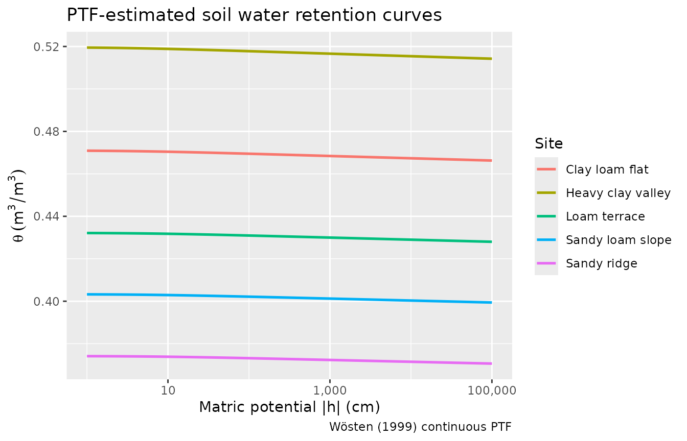
ggplot(ptf_curves, aes(x = h, y = .theta, colour = site)) +
  geom_line(linewidth = 0.9) +
  scale_x_log10(labels = scales::label_comma()) +
  labs(
    x      = "Matric potential |h| (cm)",
    y      = expression(theta~(m^3/m^3)),
    colour = "Site",
    title  = "PTF-estimated soil water retention curves",
    caption = "Wösten (1999) continuous PTF"
  )
4. Derive PAWC from PTF parameters
pawc_ptf <- ptf_params |>
tidyr::crossing(h = c(330, 15000)) |>
mutate(m = 1 - 1 / n) |>
swrc_van_genuchten(theta_r = theta_r, theta_s = theta_s,
alpha = alpha, n = n, h = h) |>
mutate(label = if_else(h == 330, "theta_fc", "theta_wp")) |>
select(site, label, .theta) |>
tidyr::pivot_wider(names_from = label, values_from = .theta) |>
mutate(pawc = theta_fc - theta_wp)
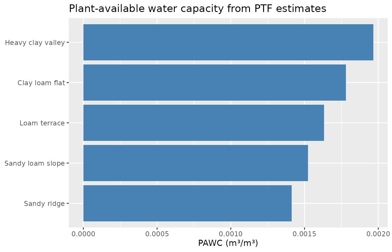
pawc_ptf |>
select(site, theta_fc, theta_wp, pawc) |>
arrange(desc(pawc))
#> # A tibble: 5 × 4
#> site theta_fc theta_wp pawc
#> <chr> <dbl> <dbl> <dbl>
#> 1 Heavy clay valley 0.517 0.515 0.00197
#> 2 Clay loam flat 0.469 0.467 0.00178
#> 3 Loam terrace 0.430 0.429 0.00163
#> 4 Sandy loam slope 0.402 0.400 0.00152
#> 5 Sandy ridge 0.373 0.371 0.00141
ggplot(pawc_ptf,
       aes(x = reorder(site, pawc), y = pawc)) +
  geom_col(fill = "steelblue") +
  coord_flip() +
  labs(
    x = NULL,
    y = "PAWC (m³/m³)",
    title = "Plant-available water capacity from PTF estimates"
  )
5. PTF vs fitted: how well do they compare?
Where measured (h, θ) data exist, it is worth comparing PTF estimates to fitted parameters.
set.seed(3109)

# Simulate lab-measured retention for the loam terrace (site 3)
loam_true <- ptf_params |> filter(site == "Loam terrace")
lab_heads  <- c(0, 10, 33, 100, 330, 1000, 5000, 15000)
lab_obs <- tibble(
  h     = lab_heads,
  theta = with(loam_true,
    theta_r + (theta_s - theta_r) /
      (1 + (alpha * lab_heads)^n)^(1 - 1/n)
  ) + rnorm(length(lab_heads), 0, 0.008)
)

# Fit VG to the simulated lab data
fitted <- fit_swrc(lab_obs, theta_col = theta, h_col = h)
#> Warning in stats::nls(formula = vg_formula, data = fit_df, start =
#> as.list(start_all), : Convergence failure: singular convergence (7)

comparison <- bind_rows(
  mutate(loam_true |> select(theta_r, theta_s, alpha, n), source = "PTF"),
  mutate(fitted     |> select(theta_r, theta_s, alpha, n), source = "Fitted")
) |>
  filter(!is.na(theta_r), theta_s > theta_r, n > 1)

comparison
#> # A tibble: 2 × 5
#>   theta_r theta_s   alpha     n source
#>     <dbl>   <dbl>   <dbl> <dbl> <chr>
#> 1   0       0.432 0.171    1.00 PTF
#> 2   0.431   0.440 0.00309 17.5  Fitted
curves_comparison <- comparison |>
  tidyr::crossing(h = heads) |>
  mutate(m = 1 - 1 / n) |>
  swrc_van_genuchten(theta_r = theta_r, theta_s = theta_s,
                     alpha = alpha, n = n, h = h)

ggplot() +
  geom_line(data  = curves_comparison,
            aes(x = h, y = .theta, colour = source, linetype = source),
            linewidth = 0.9) +
  geom_point(data = lab_obs, aes(x = h, y = theta), size = 2.5) +
  scale_x_log10(labels = scales::label_comma()) +
  labs(
    x      = "Matric potential |h| (cm)",
    y      = expression(theta~(m^3/m^3)),
    colour = "Source", linetype = "Source",
    title  = "Loam terrace: PTF estimate vs NLS fit to lab data",
    caption = "Points = simulated lab observations"
  )
#> Warning in scale_x_log10(labels = scales::label_comma()): log-10
#> transformation introduced infinite values.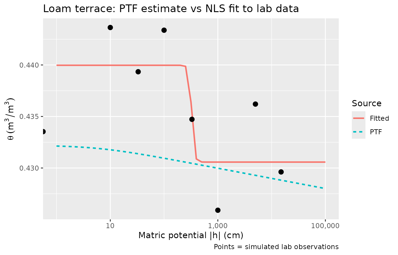
6. Real-world PTF data sources
| Source | Parameters | Coverage | Notes |
|---|---|---|---|
| Wösten et al. (1999) | θ_s, α, n, K_sat | European soils | Used in this vignette |
| Rawls & Brakensiek (1985) | θ_r, θ_s, α, n | US soils | Class-mean or continuous |
| Schaap et al. (2001) — Rosetta | θ_r, θ_s, α, n, K_sat | Global | Neural network; rosettaAPI R package |
| SoilGrids + Cosby (1984) | B-C parameters | Global 250m | Via soilDB R package |
For most applications, Rosetta 3 (Schaap 2001,
updated Zhang & Schaap 2017) provides the best accuracy for global
use. The rosettaAPI package provides access to the web
API.
Summary
The PTF workflow integrates seamlessly with
tidysoilwater:
soil_data |>
  mutate(wosten_ptf(sand, silt, clay, om, bd)) |>   # add PTF columns
  crossing(h = heads) |>
  mutate(m = 1 - 1 / n) |>
  swrc_van_genuchten(theta_r, theta_s, alpha, n, h)  # evaluate curve
PTF-derived parameters are best treated as priors — useful for rapid assessment but best validated against local laboratory data when available.