Soil water retention with swrc_van_genuchten()

library(tidysoilwater)
library(dplyr)
library(tibble)
library(ggplot2)

Overview

swrc_van_genuchten() computes the volumetric water content θ at a given matric potential h using the Van Genuchten (1980) closed-form model with the Mualem (1976) constraint (m = 1 − 1/n):

$\theta(h) = \theta_r + \frac{\theta_s - \theta_r}{\left(1 + (\alpha |h|)^n\right)^{1 - 1/n}}$

1. Parameters

Parameter	Symbol	Units	Typical range	Meaning
`theta_r`	θ_r	m³/m³	0.01 – 0.10	Residual water content
`theta_s`	θ_s	m³/m³	0.30 – 0.65	Saturated water content
`alpha`	α	1/cm	0.005 – 0.15	Inverse of air-entry pressure
`n`	n	–	1.1 – 3.5	Pore-size distribution index
`h`	h	cm	0 – 150 000	Matric potential (absolute value used)

The derived parameter m = 1 − 1/n is handled internally; you do not need to supply it.

2. Single-soil curve

# Loam soil (Carsel & Parrish 1988 typical values)
loam <- tibble(h = c(0, 10, 33, 100, 330, 1000, 3300, 5000, 10000, 15000))

loam_swrc <- swrc_van_genuchten(loam,
  theta_r = 0.078, theta_s = 0.430,
  alpha   = 0.036, n = 1.56, h = h)

loam_swrc
#> # A tibble: 10 × 2
#>        h .theta
#>    <dbl>  <dbl>
#>  1     0 0.43  
#>  2    10 0.407 
#>  3    33 0.339 
#>  4   100 0.242 
#>  5   330 0.165 
#>  6  1000 0.125 
#>  7  3300 0.102 
#>  8  5000 0.0972
#>  9 10000 0.0910
#> 10 15000 0.0884

ggplot(loam_swrc, aes(x = h, y = .theta)) +
  geom_line(linewidth = 1) +
  geom_point(size = 2.5) +
  scale_x_log10(labels = scales::label_comma()) +
  labs(
    x     = "Matric potential |h| (cm)",
    y     = expression(theta~(m^3/m^3)),
    title = "Soil water retention curve — loam"
  )
#> Warning in scale_x_log10(labels = scales::label_comma()): log-10 transformation introduced infinite values.
#> log-10 transformation introduced infinite values.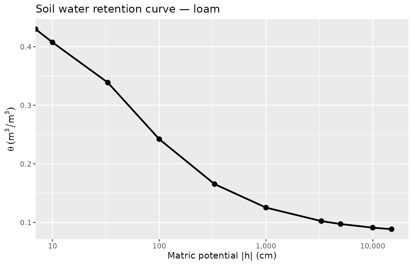

Key reference thresholds on this curve:

swrc_van_genuchten(
  tibble(h = c(0, 33, 330, 15000), label = c("saturation", "field capacity",
                                               "intermediate", "wilting point")),
  theta_r = 0.078, theta_s = 0.430,
  alpha = 0.036, n = 1.56, h = h
) |>
  select(label, h, .theta)
#> # A tibble: 4 × 3
#>   label              h .theta
#>   <chr>          <dbl>  <dbl>
#> 1 saturation         0 0.43  
#> 2 field capacity    33 0.339 
#> 3 intermediate     330 0.165 
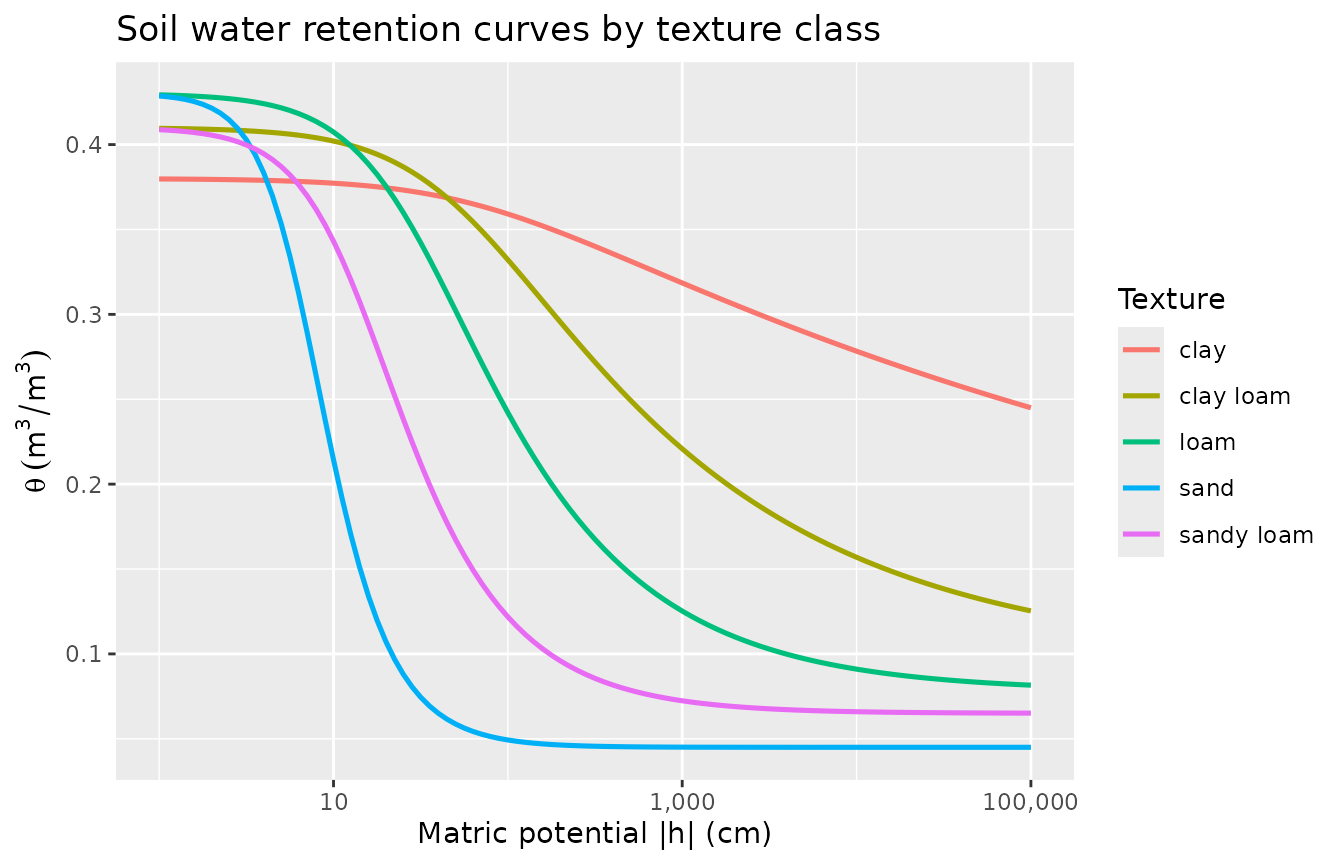
#> 4 wilting point  15000 0.0884

3. Comparing texture classes

Standard Carsel & Parrish (1988) parameters for five common texture classes:

textures <- tribble(
  ~texture,        ~theta_r, ~theta_s, ~alpha,    ~n,
  "sand",            0.045,    0.430,   0.145,  2.68,
  "sandy loam",      0.065,    0.410,   0.075,  1.89,
  "loam",            0.078,    0.430,   0.036,  1.56,
  "clay loam",       0.095,    0.410,   0.019,  1.31,
  "clay",            0.100,    0.380,   0.015,  1.09
)

heads <- 10^seq(0, 5, by = 0.05)

curves <- textures |>
  tidyr::crossing(h = heads) |>
  swrc_van_genuchten(theta_r = theta_r, theta_s = theta_s,
                     alpha = alpha, n = n, h = h)

ggplot(curves, aes(x = h, y = .theta, colour = texture)) +
  geom_line(linewidth = 0.9) +
  scale_x_log10(labels = scales::label_comma()) +
  labs(
    x      = "Matric potential |h| (cm)",
    y      = expression(theta~(m^3/m^3)),
    colour = "Texture",
    title  = "Soil water retention curves by texture class"
  )

4. Tidy evaluation: columns or scalars

All parameters accept either a bare column name from data or a scalar numeric value — mix and match as needed.

# Per-row alpha and n; scalar theta_r and theta_s
param_grid <- tibble(
  alpha = c(0.02, 0.05, 0.10, 0.15),
  n     = c(1.25, 1.50, 2.00, 2.68)
) |>
  tidyr::crossing(h = c(33, 330, 15000))

swrc_van_genuchten(param_grid,
  theta_r = 0.05,     # scalar — same for all rows
  theta_s = 0.42,     # scalar
  alpha   = alpha,    # from data column
  n       = n,        # from data column
  h       = h
) |>
  select(alpha, n, h, .theta)
#> # A tibble: 12 × 4
#>    alpha     n     h .theta
#>    <dbl> <dbl> <dbl>  <dbl>
#>  1  0.02  1.25    33 0.387 
#>  2  0.02  1.25   330 0.277 
#>  3  0.02  1.25 15000 0.139 
#>  4  0.05  1.5     33 0.303 
#>  5  0.05  1.5    330 0.141 
#>  6  0.05  1.5  15000 0.0635
#>  7  0.1   2       33 0.157 
#>  8  0.1   2      330 0.0612
#>  9  0.1   2    15000 0.0502
#> 10  0.15  2.68    33 0.0750
#> 11  0.15  2.68   330 0.0505
#> 12  0.15  2.68 15000 0.0500

5. Parameter sensitivity

Effect of α (air-entry / pore-size)

Higher α → curve drops earlier (coarser pores drain at lower suction).

tribble(
  ~alpha, ~label,
  0.005,  "α = 0.005 (fine)",
  0.02,   "α = 0.02",
  0.05,   "α = 0.05",
  0.145,  "α = 0.145 (coarse)"
) |>
  tidyr::crossing(h = heads) |>
  swrc_van_genuchten(theta_r = 0.05, theta_s = 0.42,
                     alpha = alpha, n = 1.8, h = h) |>
  ggplot(aes(x = h, y = .theta, colour = label)) +
  geom_line(linewidth = 0.9) +
  scale_x_log10(labels = scales::label_comma()) +
  labs(x = "|h| (cm)", y = expression(theta), colour = "α value",
       title = "Sensitivity to α (n fixed at 1.8)")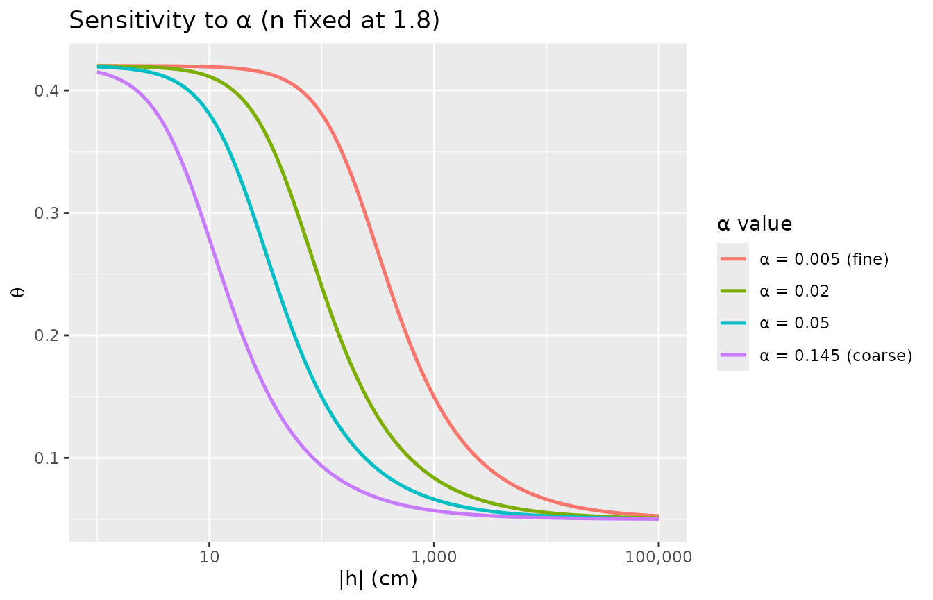

Effect of n (curve shape)

Higher n → steeper, more S-shaped curve (well-sorted pore-size distribution).

tribble(
  ~n,    ~label,
  1.10,  "n = 1.10 (clay-like)",
  1.30,  "n = 1.30",
  1.80,  "n = 1.80",
  2.68,  "n = 2.68 (sand-like)"
) |>
  tidyr::crossing(h = heads) |>
  swrc_van_genuchten(theta_r = 0.05, theta_s = 0.42,
                     alpha = 0.04, n = n, h = h) |>
  ggplot(aes(x = h, y = .theta, colour = label)) +
  geom_line(linewidth = 0.9) +
  scale_x_log10(labels = scales::label_comma()) +
  labs(x = "|h| (cm)", y = expression(theta), colour = "n value",
       title = "Sensitivity to n (α fixed at 0.04)")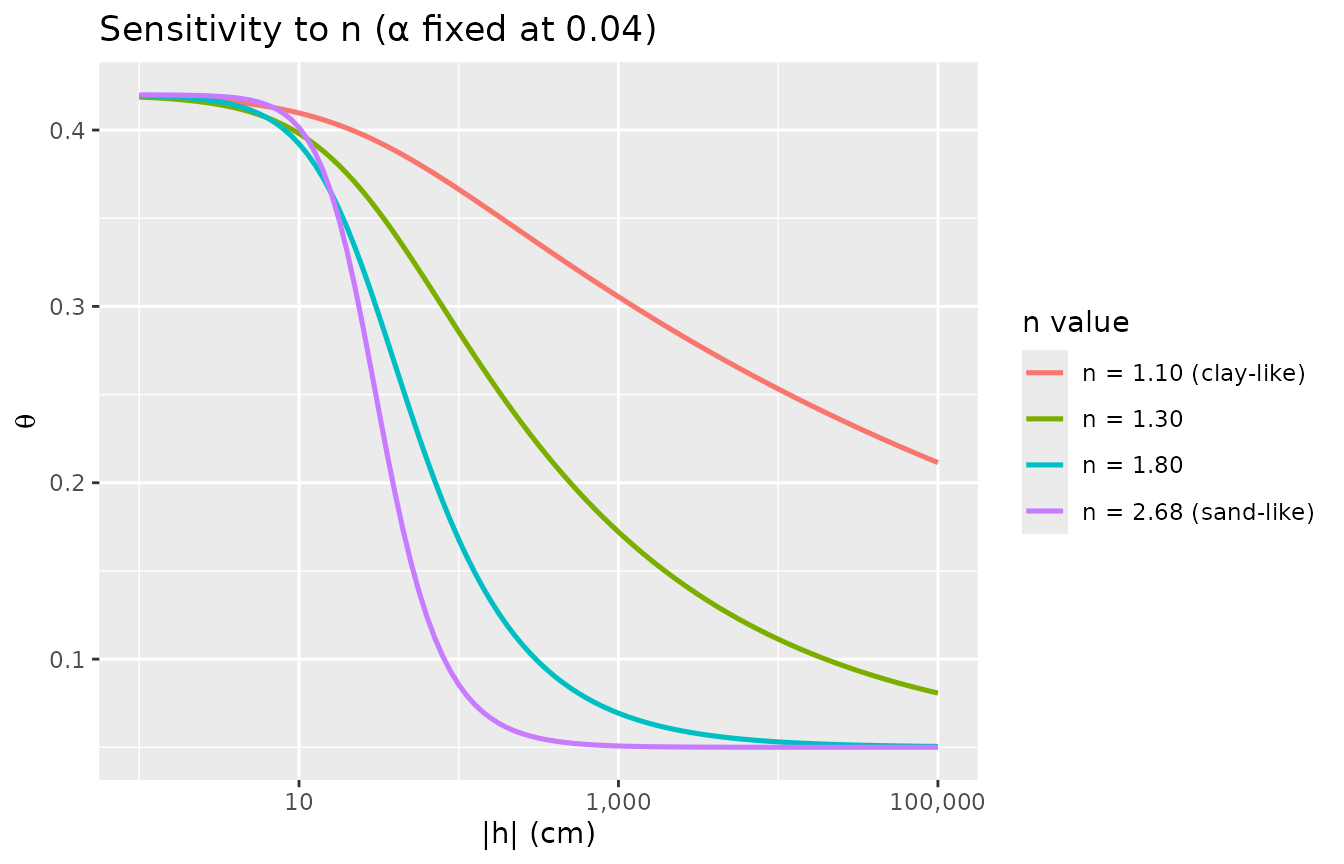

6. Sign convention

Both positive and negative h values are accepted — the absolute value is used internally. This means pF-style (positive suction) and matric potential (negative pressure) data both work without conversion.

tibble(h_negative = c(-0, -10, -100, -1000, -15000)) |>
  swrc_van_genuchten(theta_r = 0.05, theta_s = 0.42,
                     alpha = 0.04, n = 1.8, h = h_negative)
#> # A tibble: 5 × 2
#>   h_negative .theta
#>        <dbl>  <dbl>
#> 1          0 0.42  
#> 2        -10 0.392 
#> 3       -100 0.168 
#> 4      -1000 0.0693
#> 5     -15000 0.0522

7. Performance

The function uses direct tibble assignment with scalar recycling — no loops, no intermediate allocations.

df_1m <- tibble(h = rep(c(33, 330, 15000), length.out = 1e6))
elapsed <- system.time(
  swrc_van_genuchten(df_1m, theta_r = 0.05, theta_s = 0.42,
                     alpha = 0.04, n = 1.8, h = h)
)["elapsed"]
cat(sprintf("1 M rows in %.0f ms\n", elapsed * 1000))
#> 1 M rows in 41 ms