Unsaturated hydraulic conductivity with hydraulic_conductivity()

library(tidysoilwater)
library(dplyr)
library(tibble)
library(ggplot2)

Overview

hydraulic_conductivity() computes unsaturated hydraulic conductivity K(h) using the Mualem (1976) – Van Genuchten (1980) model. The effective saturation S_e is first computed from the Van Genuchten retention parameters:

$S_e(h) = \frac{1}{\left(1 + (\alpha |h|)^n\right)^m}$

Then K(h) is:

$K(h) = K_s \cdot S_e^{0.5} \cdot \left(1 - \left(1 - S_e^{1/m}\right)^m\right)^2$

where m = 1 − 1/n (the Mualem constraint). Note that m must be supplied explicitly to hydraulic_conductivity() — it is not inferred from n.

1. Parameters

Parameter	Symbol	Units	Notes
`ks`	K_s	cm/day (or any rate)	Saturated hydraulic conductivity
`alpha`	α	1/cm	Same unit system as `h`
`n`	n	–	Must be > 1
`m`	m	–	Typically `1 - 1/n`; must satisfy 0 < m < 1
`h`	h	cm	Absolute value used internally

2. Single-soil K(h) curve

# Loam soil
loam <- tibble(h = c(0, 10, 33, 100, 330, 1000, 3300, 10000, 15000))

loam_kh <- hydraulic_conductivity(loam,
  ks    = 10.4,          # cm/day (Carsel & Parrish 1988)
  alpha = 0.036,
  n     = 1.56,
  m     = 1 - 1 / 1.56,
  h     = h
)

loam_kh
#> # A tibble: 9 × 2
#>       h       .K
#>   <dbl>    <dbl>
#> 1     0 1.04e+ 1
#> 2    10 2.24e+ 0
#> 3    33 3.04e- 1
#> 4   100 1.41e- 2
#> 5   330 2.88e- 4
#> 6  1000 6.81e- 6
#> 7  3300 1.18e- 7
#> 8 10000 2.73e- 9
#> 9 15000 6.87e-10

ggplot(loam_kh, aes(x = h, y = .K)) +
  geom_line(linewidth = 1) +
  geom_point(size = 2.5) +
  scale_x_log10(labels = scales::label_comma()) +
  scale_y_log10(labels = scales::label_scientific()) +
  labs(
    x     = "Matric potential |h| (cm)",
    y     = "K(h) (cm/day)",
    title = "Unsaturated hydraulic conductivity — loam"
  )
#> Warning in scale_x_log10(labels = scales::label_comma()): log-10 transformation introduced infinite values.
#> log-10 transformation introduced infinite values.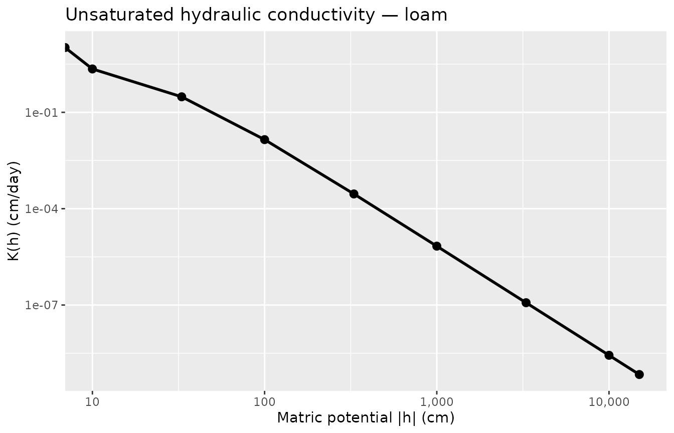

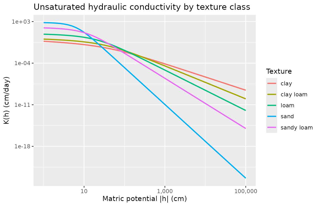
3. Comparing texture classes

Standard Carsel & Parrish (1988) parameters. K_sat values span several orders of magnitude from clay to sand.

textures <- tribble(
  ~texture,        ~ks,   ~alpha,   ~n,
  "sand",          712.8,  0.145, 2.68,
  "sandy loam",    106.1,  0.075, 1.89,
  "loam",           10.4,  0.036, 1.56,
  "clay loam",       2.2,  0.019, 1.31,
  "clay",            4.8,  0.015, 1.09
)

heads <- 10^seq(0, 5, by = 0.1)

kh_curves <- textures |>
  mutate(m = 1 - 1 / n) |>
  tidyr::crossing(h = heads) |>
  hydraulic_conductivity(ks = ks, alpha = alpha, n = n, m = m, h = h)

ggplot(kh_curves, aes(x = h, y = .K, colour = texture)) +
  geom_line(linewidth = 0.9) +
  scale_x_log10(labels = scales::label_comma()) +
  scale_y_log10(labels = scales::label_scientific()) +
  labs(
    x      = "Matric potential |h| (cm)",
    y      = "K(h) (cm/day)",
    colour = "Texture",
    title  = "Unsaturated hydraulic conductivity by texture class"
  )

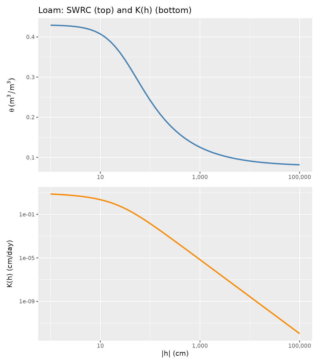
4. K(h) in context: paired SWRC and K(h) plots

K(h) and the SWRC are derived from the same parameter set. Viewing them together reveals the relationship between water storage and flow capacity.

loam_combined <- tibble(h = heads) |>
  mutate(m = 1 - 1 / 1.56) |>
  swrc_van_genuchten(theta_r = 0.078, theta_s = 0.430,
                     alpha = 0.036, n = 1.56, h = h) |>
  hydraulic_conductivity(ks = 10.4, alpha = 0.036,
                          n = 1.56, m = m, h = h)

p_theta <- ggplot(loam_combined, aes(x = h, y = .theta)) +
  geom_line(linewidth = 1, colour = "steelblue") +
  scale_x_log10(labels = scales::label_comma()) +
  labs(x = NULL, y = expression(theta~(m^3/m^3)),
       title = "Loam: SWRC (top) and K(h) (bottom)")

p_k <- ggplot(loam_combined, aes(x = h, y = .K)) +
  geom_line(linewidth = 1, colour = "darkorange") +
  scale_x_log10(labels = scales::label_comma()) +
  scale_y_log10(labels = scales::label_scientific()) +
  labs(x = "|h| (cm)", y = "K(h) (cm/day)")

# Stack with patchwork if available, otherwise print separately
if (requireNamespace("patchwork", quietly = TRUE)) {
  library(patchwork)
  p_theta / p_k
} else {
  print(p_theta)
  print(p_k)
}

5. K_sat comparison table

textures |>
  mutate(m = 1 - 1 / n) |>
  arrange(desc(ks)) |>
  select(texture, ks, alpha, n) |>
  rename(`K_sat (cm/day)` = ks,
         `α (1/cm)` = alpha)
#> # A tibble: 5 × 4
#>   texture    `K_sat (cm/day)` `α (1/cm)`     n
#>   <chr>                 <dbl>      <dbl> <dbl>
#> 1 sand                  713.       0.145  2.68
#> 2 sandy loam            106.       0.075  1.89
#> 3 loam                   10.4      0.036  1.56
#> 4 clay                    4.8      0.015  1.09
#> 5 clay loam               2.2      0.019  1.31

Note that K_sat for sand is about 150× higher than for loam, and ~650× higher than for clay loam. Even a small change in texture classification can represent a large hydraulic contrast.

6. Tidy evaluation: columns or scalars

Like swrc_van_genuchten(), all parameters accept bare column names or scalars.

# Vary K_sat and alpha across rows; scalar n and m
tibble(
  site = c("ridge", "midslope", "valley"),
  ks   = c(150, 30, 5),
  alpha = c(0.10, 0.04, 0.015)
) |>
  tidyr::crossing(h = c(10, 100, 1000)) |>
  hydraulic_conductivity(ks = ks, alpha = alpha,
                          n = 1.6, m = 1 - 1/1.6, h = h) |>
  select(site, h, alpha, ks, .K)
#> # A tibble: 9 × 5
#>   site         h alpha    ks         .K
#>   <chr>    <dbl> <dbl> <dbl>      <dbl>
#> 1 midslope    10 0.04     30 6.27      
#> 2 midslope   100 0.04     30 0.0280    
#> 3 midslope  1000 0.04     30 0.0000104 
#> 4 ridge       10 0.1     150 6.90      
#> 5 ridge      100 0.1     150 0.00642   
#> 6 ridge     1000 0.1     150 0.00000211
#> 7 valley      10 0.015     5 2.33      
#> 8 valley     100 0.015     5 0.0871    
#> 9 valley    1000 0.015     5 0.0000527

7. Performance

df_1m <- tibble(h = rep(c(33, 330, 15000), length.out = 1e6))
elapsed <- system.time(
  hydraulic_conductivity(df_1m, ks = 10, alpha = 0.036,
                          n = 1.56, m = 1 - 1/1.56, h = h)
)["elapsed"]
cat(sprintf("1 M rows in %.0f ms\n", elapsed * 1000))
#> 1 M rows in 102 ms