Multi-pedon workflow: fitting retention curves at scale • tidysoilwater

Overview

In landscape-scale soil hydrology studies, Van Genuchten parameters must be fitted independently at each sampling location (pedon). With hundreds or thousands of pedons, sequential NLS fitting becomes a throughput bottleneck. This vignette demonstrates:

Constructing a realistic multi-pedon dataset from synthetic field observations.
Running fit_swrc() sequentially and in parallel with workers = parallel::detectCores(logical = FALSE).
Mapping the fitted saturated water content (θ_s) and shape parameter (n) back to pedon locations.

Setup

library(tidysoilwater)
library(dplyr)
#> 
#> Attaching package: 'dplyr'
#> The following objects are masked from 'package:stats':
#> 
#>     filter, lag
#> The following objects are masked from 'package:base':
#> 
#>     intersect, setdiff, setequal, union
library(ggplot2)

1 Generate a synthetic pedon network

We simulate a grid of 200 pedons spread across a hypothetical study area. Each pedon is assigned one of four dominant soil textures (loam, sandy loam, clay loam, or silt loam) based on its position, mimicking the kind of spatial structure you would expect from a soil survey.

set.seed(2047)

# Van Genuchten parameters from Van Genuchten (1980, Table 1)
# Van Genuchten parameters for four textures with n > 1.5 — these are
# well-conditioned for NLS fitting.  Soils with n close to 1 (e.g. clay,
# silty clay loam) have flat retention curves that make NLS poorly
# conditioned; a real workflow would require more robust starting values
# or a Bayesian approach for those classes.
vg_reference <- tribble(
  ~texture,      ~theta_r, ~theta_s, ~alpha,  ~n,
  "sand",        0.045,    0.430,    0.145,   2.68,
  "loamy sand",  0.057,    0.410,    0.124,   2.28,
  "sandy loam",  0.065,    0.410,    0.075,   1.89,
  "loam",        0.078,    0.430,    0.036,   1.56
)

# 200 pedons on a 20 × 10 spatial grid (arbitrary units)
pedons <- expand.grid(x = seq(1, 20), y = seq(1, 10)) |>
  as_tibble() |>
  mutate(
    pedon_id = row_number(),
    # Texture follows a simple catena: coarser soils in the west,
    # finer (loam) in the east — a typical hillslope pattern
    texture = case_when(
      x <= 5  ~ "sand",
      x <= 10 ~ "loamy sand",
      x <= 15 ~ "sandy loam",
      TRUE    ~ "loam"
    )
  ) |>
  left_join(vg_reference, by = "texture")

glimpse(pedons)
#> Rows: 200
#> Columns: 8
#> $ x        <int> 1, 2, 3, 4, 5, 6, 7, 8, 9, 10, 11, 12, 13, 14, 15, 16, 17, 18…
#> $ y        <int> 1, 1, 1, 1, 1, 1, 1, 1, 1, 1, 1, 1, 1, 1, 1, 1, 1, 1, 1, 1, 2…
#> $ pedon_id <int> 1, 2, 3, 4, 5, 6, 7, 8, 9, 10, 11, 12, 13, 14, 15, 16, 17, 18…
#> $ texture  <chr> "sand", "sand", "sand", "sand", "sand", "loamy sand", "loamy …
#> $ theta_r  <dbl> 0.045, 0.045, 0.045, 0.045, 0.045, 0.057, 0.057, 0.057, 0.057…
#> $ theta_s  <dbl> 0.43, 0.43, 0.43, 0.43, 0.43, 0.41, 0.41, 0.41, 0.41, 0.41, 0…
#> $ alpha    <dbl> 0.145, 0.145, 0.145, 0.145, 0.145, 0.124, 0.124, 0.124, 0.124…
#> $ n        <dbl> 2.68, 2.68, 2.68, 2.68, 2.68, 2.28, 2.28, 2.28, 2.28, 2.28, 1…

2 Simulate field observations

Laboratory or field tensiometer measurements typically cover 8–12 pressure heads from saturation (h = 0) to permanent wilting point (h = 15 000 cm). We generate synthetic θ(h) observations by evaluating the VG model at each pedon’s true parameters, then adding realistic measurement noise (σ = 0.005 m³/m³).

h_obs <- c(0, 1, 5, 10, 50, 100, 300, 500, 1000, 3000, 5000, 15000)

# Each row of pedons becomes a set of (h, theta) observations
obs_data <- pedons |>
  rowwise() |>
  mutate(
    # Slight spatial heterogeneity: jitter parameters within ±10 %
    alpha_loc   = alpha   * runif(1, 0.90, 1.10),
    n_loc       = max(1.05, n * runif(1, 0.90, 1.10)),
    theta_r_loc = theta_r * runif(1, 0.90, 1.10),
    theta_s_loc = theta_s * runif(1, 0.90, 1.10),
    obs = list({
      theta_true <- swrc_van_genuchten(
        tibble(h = h_obs),
        theta_r = theta_r_loc, theta_s = theta_s_loc,
        alpha   = alpha_loc,   n       = n_loc,
        h       = h
      )$.theta
      tibble(
        h     = h_obs,
        theta = pmax(0, theta_true + rnorm(length(h_obs), sd = 0.005))
      )
    })
  ) |>
  tidyr::unnest(obs) |>
  ungroup()

cat(sprintf("%d pedons × %d pressure heads = %d observations total\n",
            n_distinct(obs_data$pedon_id),
            length(h_obs),
            nrow(obs_data)))
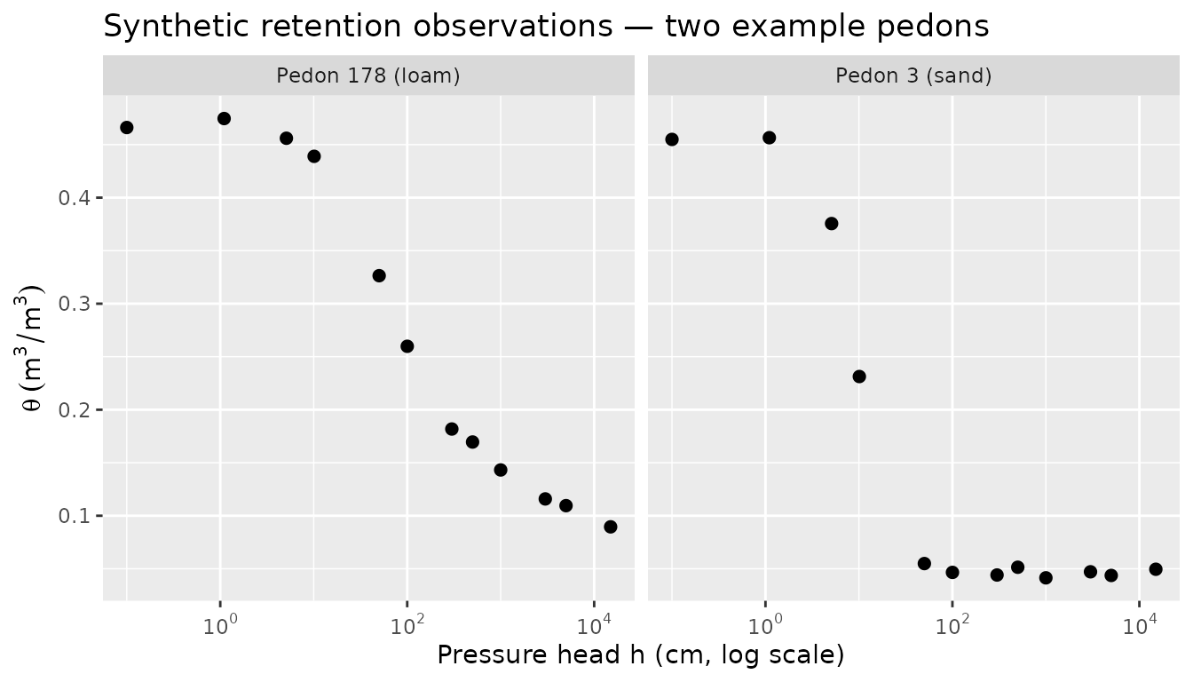
#> 200 pedons × 12 pressure heads = 2400 observations total

Spot-check two pedons from contrasting texture zones:

filter(obs_data, pedon_id %in% c(3, 178)) |>
  mutate(label = paste0("Pedon ", pedon_id, " (", texture, ")")) |>
  ggplot(aes(h + 0.1, theta)) +
  geom_point(size = 2) +
  scale_x_log10(labels = scales::label_log()) +
  facet_wrap(~label) +
  labs(
    x = "Pressure head h (cm, log scale)",
    y = expression(theta~(m^3/m^3)),
    title = "Synthetic retention observations — two example pedons"
  )

Retention curves for two pedons with contrasting soil textures

3 Fit Van Genuchten parameters per pedon

3.1 Sequential baseline

t_seq <- system.time(
  fits_seq <- suppressWarnings(
    obs_data |>
      group_by(pedon_id, x, y, texture) |>
      fit_swrc(theta_col = theta, h_col = h, workers = 1L)
  )
)["elapsed"]

cat(sprintf("Sequential: %.2f s for %d pedons (%.1f ms / pedon)\n",
            t_seq, nrow(fits_seq), t_seq / nrow(fits_seq) * 1000))
#> Sequential: 0.86 s for 200 pedons (4.3 ms / pedon)
cat(sprintf("Converged: %d / %d (%.0f %%)\n",
            sum(fits_seq$convergence),
            nrow(fits_seq),
            mean(fits_seq$convergence) * 100))
#> Converged: 200 / 200 (100 %)

3.2 Parallel fit with all physical cores

# R CMD check restricts parallel forking; cap to 2 in that environment
in_check <- isTRUE(as.logical(Sys.getenv("_R_CHECK_LIMIT_CORES_", "FALSE")))
n_cores  <- if (in_check) 2L else parallel::detectCores(logical = FALSE)
cat(sprintf("Workers used: %d\n", n_cores))
#> Workers used: 4

t_par <- system.time(
  fits_par <- suppressWarnings(
    obs_data |>
      group_by(pedon_id, x, y, texture) |>
      fit_swrc(theta_col = theta, h_col = h, workers = n_cores)
  )
)["elapsed"]

cat(sprintf("Parallel (%d workers): %.2f s — speedup %.1fx\n",
            n_cores, t_par, t_seq / t_par))
#> Parallel (4 workers): 0.54 s — speedup 1.6x

3.3 Verify consistency

The sequential and parallel paths run identical NLS fits; parameter estimates must match to machine precision.

fits_seq_ord <- arrange(fits_seq, pedon_id)
fits_par_ord <- arrange(fits_par, pedon_id)

max_diff_theta_s <- max(abs(fits_seq_ord$theta_s - fits_par_ord$theta_s),
                        na.rm = TRUE)
max_diff_alpha   <- max(abs(fits_seq_ord$alpha   - fits_par_ord$alpha),
                        na.rm = TRUE)

cat(sprintf("Max |Δθ_s| seq vs par: %.2e\n", max_diff_theta_s))
#> Max |Δθ_s| seq vs par: 0.00e+00
cat(sprintf("Max |Δα|   seq vs par: %.2e\n", max_diff_alpha))
#> Max |Δα|   seq vs par: 0.00e+00
stopifnot(max_diff_theta_s < 1e-8, max_diff_alpha < 1e-8)

4 Map fitted parameters

With 200 pedons on a regular grid, we can visualise how the fitted θ_s and shape parameter n vary across the landscape.

fits_seq |>
  filter(convergence) |>
  ggplot(aes(x, y, fill = theta_s)) +
  geom_tile(width = 0.95, height = 0.95) +
  scale_fill_distiller(palette = "Blues", direction = 1,
                       name = expression(theta[s]~(m^3/m^3))) +
  coord_equal() +
  labs(
    title = "Fitted saturated water content (θ_s) across the study area",
    x = "Easting (arbitrary)", y = "Northing (arbitrary)"
  ) +
  theme_minimal()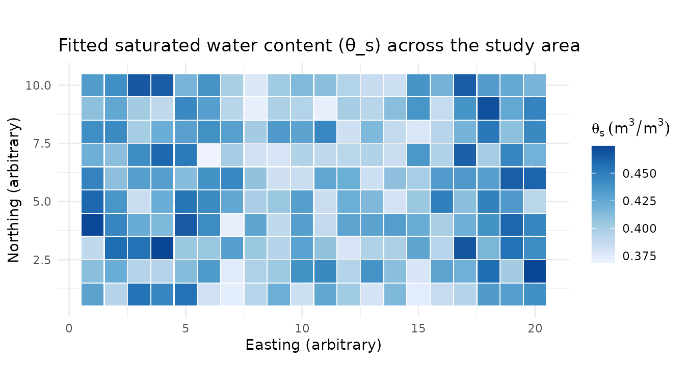

Spatial map of fitted saturated water content

fits_seq |>
  filter(convergence) |>
  ggplot(aes(x, y, fill = n)) +
  geom_tile(width = 0.95, height = 0.95) +
  scale_fill_distiller(palette = "RdYlBu", direction = 1,
                       name = "n (−)") +
  coord_equal() +
  labs(
    title = "Fitted Van Genuchten shape parameter n",
    subtitle = "Sandy soils (left) have higher n than clay soils (centre-right)",
    x = "Easting (arbitrary)", y = "Northing (arbitrary)"
  ) +
  theme_minimal()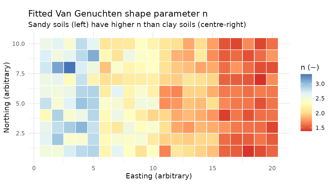

Spatial map of fitted Van Genuchten shape parameter n

5 Spatial integration with sf (optional)

When pedon coordinates are in a real CRS, the fitted parameters can be attached directly to an sf point layer for further geostatistical analysis or export as GeoPackage / Shapefile.

pedons_sf <- fits_seq |>
  filter(convergence) |>
  sf::st_as_sf(coords = c("x", "y"), crs = NA_integer_)

# Inspect: each feature carries fitted VG parameters
print(pedons_sf[1:4, c("texture", "theta_r", "theta_s", "alpha", "n")])
#> Simple feature collection with 4 features and 5 fields
#> Geometry type: POINT
#> Dimension:     XY
#> Bounding box:  xmin: 1 ymin: 1 xmax: 4 ymax: 1
#> CRS:           NA
#> # A tibble: 4 × 6
#>   texture theta_r theta_s alpha     n geometry
#>   <chr>     <dbl>   <dbl> <dbl> <dbl>  <POINT>
#> 1 sand     0.0471   0.429 0.157  2.52    (1 1)
#> 2 sand     0.0431   0.393 0.148  2.49    (2 1)
#> 3 sand     0.0450   0.456 0.142  2.71    (3 1)
#> 4 sand     0.0446   0.445 0.143  2.83    (4 1)

With a real CRS you can then write:

sf::st_write(pedons_sf, "fitted_vg_params.gpkg")

6 Real-world data sources

In practice, the obs_data tibble would be built from one of these sources:

Source	Format	Typical h range	θ unit
Hypres / UNSODA	CSV	0–15 000 cm	m³/m³
SoilGrids point extraction	JSON / raster	—	volumetric fraction
Field tensiometer loggers	CSV / NetCDF	0–800 hPa	m³/m³ or %
Laboratory pressure-plate	CSV	0–15 000 cm	m³/m³

Convert pressure in hPa to cm water head with the approximation 1 hPa ≈ 1.02 cm H₂O.

Summary

Multi-pedon workflow steps
Step	Code
Generate observations	swrc_van_genuchten() per pedon
Sequential fit (baseline)	group_by(pedon_id) \|> fit_swrc(workers = 1)
Parallel fit	fit_swrc(workers = parallel::detectCores(logical = FALSE))
Attach to spatial layer	sf::st_as_sf(fits, coords = c(‘x’,‘y’), crs = …)
Export	sf::st_write(pedons_sf, ‘fitted_vg.gpkg’)