Raster workflow: mapping soil hydraulic properties • tidysoilwater

library(tidysoilwater)
library(dplyr)
library(tidyr)
library(tibble)
library(ggplot2)

Overview

Soil hydraulic properties vary continuously across the landscape. This vignette shows how to:

Build a spatial grid with spatially varying Van Genuchten parameters
Evaluate the SWRC and K(h) at multiple pressure heads for every grid cell
Derive plant-available water capacity (PAWC)
Map results using ggplot2 (and optionally export to a terra SpatRaster)

The approach works with any data source: SoilGrids-derived PTF estimates, field-fitted parameters stored in a database, or synthetic parameter maps.

1. Build a spatial parameter grid

We construct a 50 × 50 grid (2 500 cells) representing a hillslope transect from sandy ridge soils to loamy valley soils. Van Genuchten parameters vary linearly with a topographic wetness index proxy (twi).

set.seed(8831)
n_x <- 50L
n_y <- 50L

grid <- expand.grid(x = seq_len(n_x), y = seq_len(n_y)) |>
  as_tibble() |>
  mutate(
    # Topographic wetness proxy: higher near valley (small x)
    twi   = (n_x - x) / n_x + rnorm(n(), 0, 0.05),
    twi   = pmax(0, pmin(1, twi)),

    # Parameters shift from sandy (low twi) to loamy (high twi)
    theta_r = 0.03  + 0.04  * twi,
    theta_s = 0.35  + 0.12  * twi,
    alpha   = 0.10  - 0.06  * twi,   # coarser pores → higher alpha
    n       = 2.50  - 0.90  * twi,   # coarser texture → higher n
    ks      = 200   * exp(-3 * twi)  # K_sat decreases toward valley
  )

glimpse(grid)
#> Rows: 2,500
#> Columns: 8
#> $ x       <int> 1, 2, 3, 4, 5, 6, 7, 8, 9, 10, 11, 12, 13, 14, 15, 16, 17, 18,…
#> $ y       <int> 1, 1, 1, 1, 1, 1, 1, 1, 1, 1, 1, 1, 1, 1, 1, 1, 1, 1, 1, 1, 1,…
#> $ twi     <dbl> 0.8507768, 1.0000000, 0.9624511, 0.8597789, 0.9271878, 0.78772…
#> $ theta_r <dbl> 0.06403107, 0.07000000, 0.06849804, 0.06439116, 0.06708751, 0.…
#> $ theta_s <dbl> 0.4520932, 0.4700000, 0.4654941, 0.4531735, 0.4612625, 0.44452…
#> $ alpha   <dbl> 0.04895339, 0.04000000, 0.04225294, 0.04841327, 0.04436873, 0.…
#> $ n       <dbl> 1.734301, 1.600000, 1.633794, 1.726199, 1.665531, 1.791043, 1.…
#> $ ks      <dbl> 15.579984, 9.957414, 11.144701, 15.164856, 12.388317, 18.82391…

2. Evaluate SWRC at multiple pressure heads

We evaluate θ(h) at 12 standard pressure heads, producing a long-format tibble — one row per grid cell per head value.

heads <- c(0, 10, 33, 100, 330, 1000, 3300, 5000, 10000, 15000)

swrc_long <- grid |>
  tidyr::crossing(h = heads) |>
  swrc_van_genuchten(
    theta_r = theta_r,
    theta_s = theta_s,
    alpha   = alpha,
    n       = n,
    h       = h
  )

cat(sprintf("Rows: %d  (%.0f cells × %d heads)\n",
            nrow(swrc_long), n_x * n_y, length(heads)))
#> Rows: 25000  (2500 cells × 10 heads)

SWRC curves: ridge vs valley

# Sample a ridge cell (x=48) and a valley cell (x=2)
example_cells <- swrc_long |>
  filter(x %in% c(2, 48), y == 25) |>
  mutate(position = if_else(x == 2, "Valley (loam)", "Ridge (sandy loam)"))

ggplot(example_cells, aes(x = h, y = .theta, colour = position)) +
  geom_line(linewidth = 1) +
  scale_x_log10(
    labels = scales::label_comma(),
    breaks = c(1, 10, 100, 1000, 10000)
  ) +
  labs(
    x      = "Matric potential |h| (cm)",
    y      = expression(theta~(m^3/m^3)),
    colour = NULL,
    title  = "Soil water retention curves: ridge vs valley"
  )
#> Warning in scale_x_log10(labels = scales::label_comma(), breaks = c(1, 10, :
#> log-10 transformation introduced infinite values.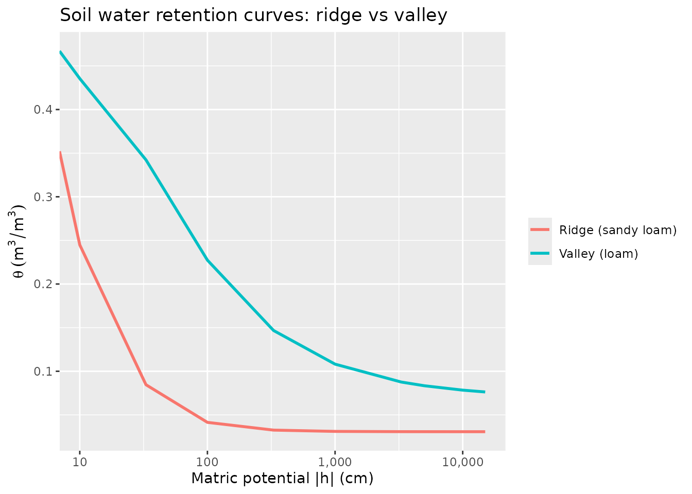

3. Derive plant-available water capacity

PAWC = θ at field capacity (|h| = 330 cm, pF 2.5) minus θ at wilting point (|h| = 15 000 cm, pF 4.2). Both heads are already in our long-format tibble.

water_map <- swrc_long |>
  filter(h %in% c(330, 15000)) |>
  mutate(label = if_else(h == 330, "theta_fc", "theta_wp")) |>
  select(x, y, label, .theta) |>
  tidyr::pivot_wider(names_from = label, values_from = .theta) |>
  mutate(
    pawc    = theta_fc - theta_wp,
    theta_s = grid$theta_s[match(paste(x, y), paste(grid$x, grid$y))]
  )

summary(water_map[c("theta_fc", "theta_wp", "pawc")])
#>     theta_fc          theta_wp            pawc         
#>  Min.   :0.03169   Min.   :0.03001   Min.   :0.001682  
#>  1st Qu.:0.04416   1st Qu.:0.03957   1st Qu.:0.004584  
#>  Median :0.06284   Median :0.05003   Median :0.012809  
#>  Mean   :0.07149   Mean   :0.05080   Mean   :0.020699  
#>  3rd Qu.:0.09286   3rd Qu.:0.06094   3rd Qu.:0.031924  
#>  Max.   :0.15455   Max.   :0.07861   Max.   :0.075937

Map PAWC across the grid

ggplot(water_map, aes(x = x, y = y, fill = pawc)) +
  geom_tile() +
  scale_fill_distiller(
    palette  = "Blues",
    direction = 1,
    name     = "PAWC\n(m³/m³)"
  ) +
  coord_equal() +
  labs(
    title    = "Plant-available water capacity",
    subtitle = "Sandy ridge (right) → loamy valley (left)",
    x = "x (grid column)", y = "y (grid row)"
  ) +
  theme_minimal()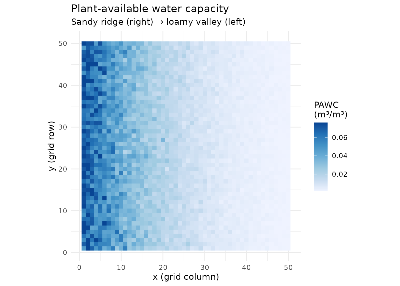

4. Evaluate K(h) across the grid

kh_long <- grid |>
  tidyr::crossing(h = heads[-1]) |>   # exclude h=0 (K_sat = ks directly)
  mutate(m = 1 - 1 / n) |>
  hydraulic_conductivity(
    ks    = ks,
    alpha = alpha,
    n     = n,
    m     = m,
    h     = h
  )

cat(sprintf("K(h) rows: %d\n", nrow(kh_long)))
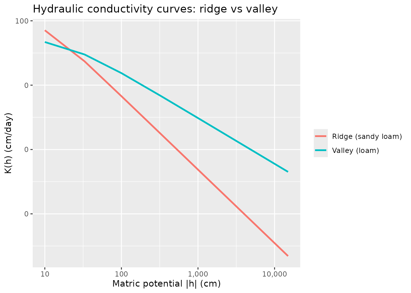
#> K(h) rows: 22500

K(h) curves: ridge vs valley

kh_long |>
  filter(x %in% c(2, 48), y == 25) |>
  mutate(position = if_else(x == 2, "Valley (loam)", "Ridge (sandy loam)")) |>
  ggplot(aes(x = h, y = .K, colour = position)) +
  geom_line(linewidth = 1) +
  scale_x_log10(labels = scales::label_comma()) +
  scale_y_log10(labels = scales::label_comma()) +
  labs(
    x      = "Matric potential |h| (cm)",
    y      = "K(h) (cm/day)",
    colour = NULL,
    title  = "Hydraulic conductivity curves: ridge vs valley"
  )

Map K at field capacity

k_fc <- kh_long |>
  filter(h == 330) |>
  select(x, y, K_fc = .K)

ggplot(k_fc, aes(x = x, y = y, fill = log10(K_fc))) +
  geom_tile() +
  scale_fill_distiller(
    palette   = "Oranges",
    direction = 1,
    name      = "log₁₀ K(fc)\n(cm/day)"
  ) +
  coord_equal() +
  labs(
    title    = "Hydraulic conductivity at field capacity",
    subtitle = "Sandy ridge (right) → loamy valley (left)",
    x = "x", y = "y"
  ) +
  theme_minimal()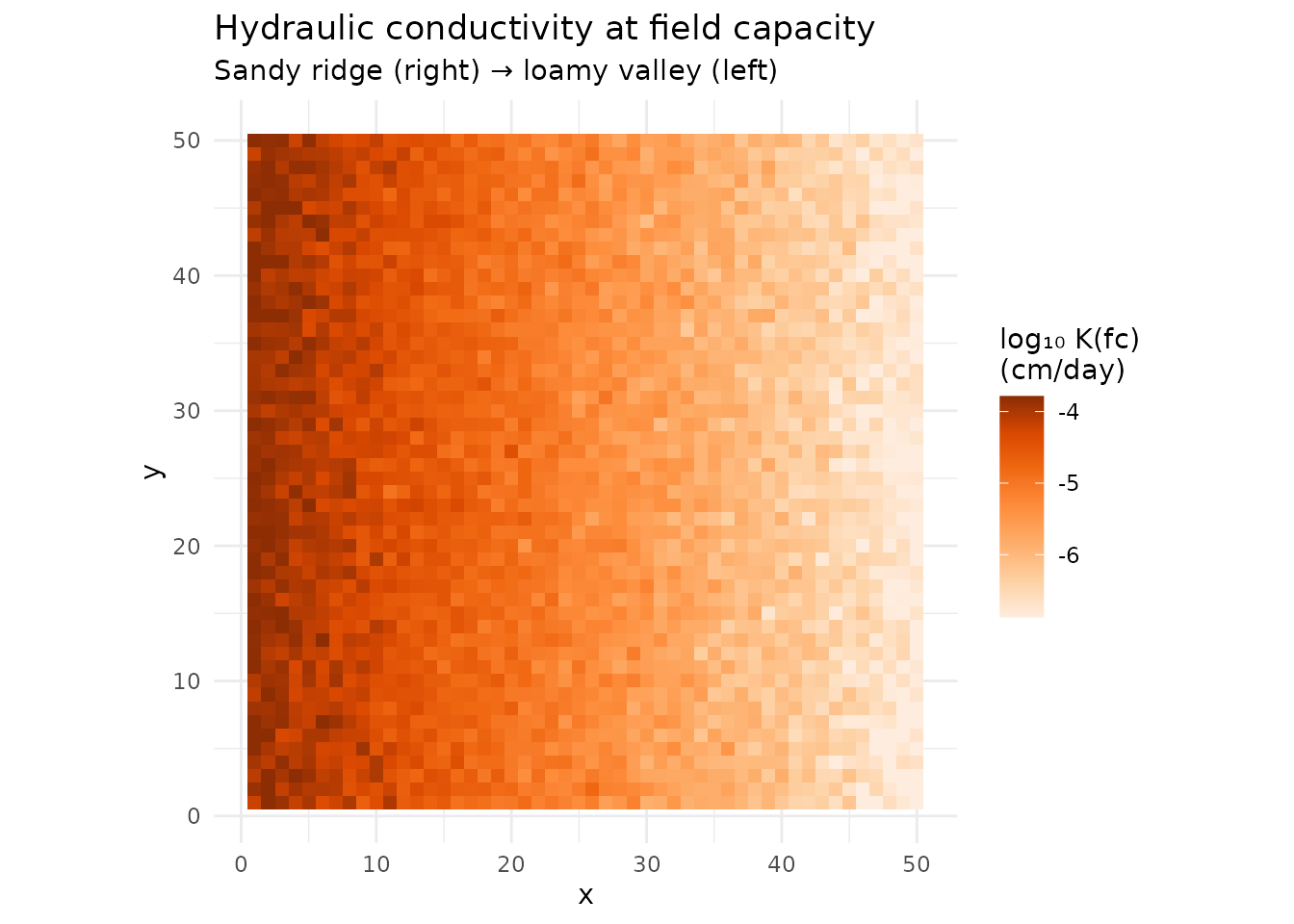

5. Export to terra SpatRaster (optional)

If terra is available, the grid tibble converts directly to a multi-layer raster for further GIS analysis or output.

library(terra)

# Combine scalar water properties into a wide summary
raster_df <- water_map |>
  left_join(k_fc, by = c("x", "y")) |>
  arrange(y, x)

r_out <- terra::rast(
  ncols = n_x, nrows = n_y,
  xmin = 0, xmax = n_x, ymin = 0, ymax = n_y
)
r_out <- c(
  terra::setValues(r_out, raster_df$theta_fc),
  terra::setValues(r_out, raster_df$theta_wp),
  terra::setValues(r_out, raster_df$pawc),
  terra::setValues(r_out, log10(raster_df$K_fc))
)
names(r_out) <- c("theta_fc", "theta_wp", "pawc", "log10_K_fc")

print(r_out)

#> terra not installed — skipping SpatRaster export section.

Summary

Step	Function	Output
SWRC across grid	`swrc_van_genuchten()`	θ(h) for all cells × heads
Derive PAWC	`pivot_wider()` + mutate	θ_fc, θ_wp, PAWC per cell
K(h) across grid	`hydraulic_conductivity()`	K(h) for all cells × heads
Raster export	`terra::rast()`	Multi-layer GeoTIFF

The key pattern is expand.grid() (or tidyr::crossing()) to broadcast parameters across head values, then pass the result directly to swrc_van_genuchten() or hydraulic_conductivity() — no loops needed.